CQC Intros: Quantum Computing

Civilisation has advanced as people discovered new ways of exploiting various physical resources such as materials, forces and energies. In the twentieth century information was added to the list when the invention of computers allowed complex information processing to be performed outside human brains. The history of computer technology has involved a sequence of changes from one type of physical realisation to another --- from gears to relays to valves to transistors to integrated circuits and so on. Today's advanced lithographic techniques can squeeze fraction of micron wide logic gates and wires onto the surface of silicon chips. Soon they will yield even smaller parts and inevitably reach a point where logic gates are so small that they are made out of only a handful of atoms. On the atomic scale matter obeys the rules of quantum mechanics, which are quite different from the classical rules that determine the properties of conventional logic gates. So if computers are to become smaller in the future, new, quantum technology must replace or supplement what we have now. The point is, however, that quantum technology can offer much more than cramming more and more bits to silicon and multiplying the clock-speed of microprocessors. It can support entirely new kind of computation with qualitatively new algorithms based on quantum principles!

To explain what makes quantum computers so different from their classical counterparts we begin by having a closer look at a basic chunk of information namely one bit. From a physical point of view a bit is a physical system which can be prepared in one of the two different states representing two logical values --- no or yes, false or true, or simply 0 or

1. For example, in digital computers, the voltage between the plates in a capacitor represents a bit of information: a charged capacitor denotes bit value 1 and an uncharged capacitor bit value 0. One bit of information can be also encoded using two different polarisations of light or two different electronic states of an atom. However, if we choose an atom as a physical bit then quantum mechanics tells us that apart from the two distinct electronic states the atom can be also prepared in a coherent superposition of the two states. This means that the atom is both in state 0 and state 1. To get used to the idea that a quantum object can be in `two states at once' it is helpful to consider the following experiment (Fig.A and B)

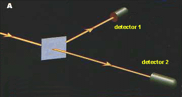Let us try to reflect a single photon off a half-silvered mirror i.e. a mirror which reflects exactly half of the light which impinges upon it, while the remaining half is transmitted directly through it (Fig. A). Where do you think the photon is after its encounter with the mirror --- is it in the reflected or in the transmitted beam? It seems that it would be sensible to say that the photon is either in the transmitted or in the reflected beam with the same probability. That is one might expect the photon to take one of the two paths choosing randomly which way to go. Indeed, if we place two photodetectors behind the half-silvered mirror in direct lines of the two beams, the photon will be registered with the same probability

either in the detector 1 or in the detector 2. Does it really mean that after the half-silvered mirror the photon travels in either reflected or transmitted beam with the same probability 50%? No, it does not ! In fact the photon takes `two paths at once'. This can be demonstrated by recombining the two beams with the help of two fully silvered mirrors and placing another half-silvered mirror at their meeting point, with two photodectors in direct lines of the two beams (Fig. B). With this set up we can observe a truly amazing quantum interference phenomenon.

If it were merely the case that there were a 50% chance that the photon followed one path and a 50% chance that it followed the other, then we should find a 50% probability that one of the detectors registers the photon and a 50% probability that the other one does. However, that is not what happens. If the two possible paths are exactly equal in length, then it turns out that there is a 100% probability that the photon reaches the detector 1 and 0% probability that it reaches the other detector 2. Thus the photon is certain to strike the detector 1! It seems inescapable that the photon must, in some sense, have actually travelled both routes at once for if an absorbing screen is placed in the way of either of the two routes, then it becomes equally probable that detector 1 or 2 is reached (Fig. 1c). Blocking off one of the paths actually allows B to be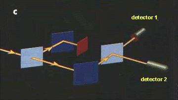

reached; with both routes open, the photon somehow knows that it is not permitted to reach detector2, so it must have actually felt out both routes. It is therefore perfectly legitimate to say that between the two half-silvered mirrors the photon took both the transmitted and the reflected paths or, using more technical language, we can say that the photon is in a coherent superposition of being in the transmitted beam and in the reflected beam. By the same token an atom can be prepared in a superposition of two different electronic states, and in general a quantum two state system, called a quantum bit or a qubit, can be prepared in a superposition of its two logical states 0 and 1. Thus one qubit can encode at a given moment of time both 0 and 1.

Now we push the idea of superposition of numbers a bit further. Consider a register composed of three physical bits. Any classical register of that type can store in a given moment of time only one out of eight different numbers i.e the register can be in only one out of eight possible configurations such as 000, 001, 010, ... 111. A quantum register composed of three qubits can store in a given moment of time all eight numbers in a quantum superposition (Fig. 2). This is quite remarkable that all eight numbers are physically present in the register but it should be no more surprising than a qubit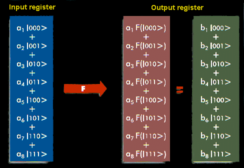

being both in state 0 and 1 at the same time. If we keep adding qubits to the register we increase its storage capacity exponentially i.e. three qubits can store 8 different numbers at once, four qubits can store 16 different numbers at once, and so on; in general L qubits can store 2^L numbers at once. Once the register is prepared in a superposition of different numbers we can perform operations on all of them. For example, if qubits are atoms then suitably tuned laser pulses affect atomic electronic states and evolve initial superpositions of encoded numbers into different superpositions. During such evolution each number in the superposition is affected and as the result we generate a massive parallel computation albeit in one piece of quantum hardware. This means that a quantum computer can in only one computational step perform the same mathematical operation on 2^L different input numbers encoded in coherent superpositions of L qubits. In order to acomplish the same task any classical computer has to repeat the same computation 2^L times or one has to use 2^L different processors working in parallel. In other words a quantum computer offers an enormous gain in the use of computational resources such as time and memory.

But this, after all, sounds as yet another purely technological progress. It looks like classical computers can do the same computations as quantum computers but simply need more time or more memory. The catch is that classical computers need exponentially more time or memory to match the power of quantum computers and this is really asking for too much because an exponential increase is really fast and we run out of available time or memory very quickly. Let us have a closer look at this issue.

In order to solve a particular problem computers follow a precise set of instructions that can be mechanically applied to yield the solution to any given instance of the problem. A specification of this set of instructions is called an algorithm. Examples of algorithms are the procedures taught in elementary schools for adding and multiplying whole numbers; when these procedures are mechanically applied, they always yield the correct result for any pair of whole numbers. Some algorithms are fast (e.g. multiplication) other are very slow (e.g. factorisation, playing chess). Consider, for example, the following factorisation problem

How long would it take you, using paper and pencil, to find the two whole numbers which should be written into the two boxes (the solution is unique)? Probably about one hour. Solving the reverse problem

again using paper and pencil technique, takes less than a minute. All because we know fast algorithms for multiplication but we do not know equally fast ones for factorisation. What really counts for a ``fast'' or a ``usable'' algorithm, according to the standard definition, is not the actual time taken to multiply a particular pairs of number but the fact that the time does not increase too sharply when we apply the same method to ever larger numbers. The same standard text-book method of multiplication requires little extra work when we switch from two three digit numbers to two thirty digits numbers. By contrast, factoring a thirty digit number using the simplest trial divison method (see inset 1) is about 10¹³ times more time or memory consuming than factoring a three digit number. The use of computational resources is enormous when we keep increasing the number of digits. The largest number that has been factorised as a mathematical challenge, i.e. a number whose factors were secretly chosen by mathematicians in order to present a challenge to other mathematicians, had 129 digits. No one can even conceive of how one might factorise say thousand-digit numbers; the computation would take much more that the estimated age of the universe.

Skipping details of the computational complexity we only mention that computer scientists have a rigorous way of defining what makes an algorithm fast (and usable) or slow (and unusable). For an algorithm to be fast, the time it takes to execute the algorithm must increase no faster than a polynomial function of the size of the input. Informally think about the input size as the total number of bits needed to specify the input to the problem, for example, the number of bits needed to encode the number we want to factorise. If the best algorithm we know for a particular problem has the execution time (viewed as a function of the size of the input) bounded by a polynomial then we say that the problem belongs to class P. Problems outside class P are known as hard problems. Thus we say, for example, that multiplication is in P whereas factorisation is not in P and that is why it is a hard problem. Hard does not mean ``impossible to solve'' or ``non-computable'' --- factorisation is perfectly computable using a classical computer, however, the physical resources needed to factor a large number are such that for all practical purposes, it can be regarded as intractable (see inset 1).

It worth pointing out that computer scientists have carefully constructed the definitions of efficient and inefficient algorithms trying to avoid any reference to a physical hardware. According to the above definition factorisation is a hard problem for any classical computer regardless its make and the clock-speed. Have a look at Fig.3 and compare a modern computer with its ancestor of the nineteenth century, the Babbage differential engine. The technological gap is obvious and yet the Babbage engine can perform the same computations as the modern digital computer. Moreover, factoring is equally difficult both for the Babbage engine and top-of-the-line connection machine; the execution time grows exponentially with the size of the number in both cases. Thus purely technological progress can only increase the computational speed by a fixed multiplicative factor which does not help to change the exponential dependance between the size of the input and the execution time. Such change requires inventing new, better algorithms. Although quantum computation requires new quantum technology its real power lies in new quantum algorithms which allow to exploit quantum superposition that can contain an exponential number of different terms. Quantum computers can be programed in a qualitatively new way. For example, a quantum program can incorporate instructions such as `... and now take a superposition of all numbers from the previous operations...'; this instruction is meaningless for any classical data processing device but makes lots of sense to a quantum computer. As the result we can construct new algorithms for solving problems, some of which can turn difficult mathematical problems, such as factorisation, into easy ones!

The story of quantum computation started as early as 1982, when the physicist Richard Feynman considered simulation of quantum-mechanical objects by other quantum systems[1]. However, the unusual power of quantum computation was not really anticipated untill the 1985 when David Deutsch of the University of Oxford published a crucial theoretical paper[2] in which he described a universal quantum computer. After the Deutsch paper, the hunt was on for something interesting for quantum computers to do. At the time all that could be found were a few rather contrived mathematical problems and the whole issue of quantum computation seemed little more than an academic curiosity. It all changed rather suddenly in 1994 when Peter Shor from AT&T's Bell Laboratories in New Jersey devised the first quantum algorithm that, in principle, can perform efficient factorisation[3].This became a `killer application' --- something very useful that only a quantum computer could do. Difficulty of factorisation underpins security of many common methods of encryption; for example, RSA --- the most popular public key cryptosystem which is often used to protect electronic bank accounts gets its security from the difficulty of factoring large numbers. Potential use of quantum computation for code-breaking purposes has raised an obvious question --- what about building a quantum computer.

In principle we know how to build a quantum computer; we can start with simple quantum logic gates and try to integrate them together into quantum circuits. A quantum logic gate, like a classical gate, is a very simple computing device that performs one elementary quantum operation, usually on two qubits, in a given period of time[4]. Of course, quantum logic gates are different from their classical counterparts because they can create and perform operations on quantum superpositions (cf. inset 2). However if we keep on putting quantum gates together into circuits we will quickly run into some serious practical problems. The more interacting qubits are involved the harder it tends to be to engineer the interaction that would display the quantum interference. Apart from the technical difficulties of working at single-atom and single-photon scales, one of the most important problems is that of preventing the surrounding environment from being affected by the interactions that generate quantum superpositions. The more components the more likely it is that quantum computation will spread outside the computational unit and will irreversibly dissipate useful information to the environment. This process is called decoherence. Thus the race is to engineer sub-microscopic systems in which qubits interact only with themselves but not not with the environment.

Some physicists are pessimistic about the prospects of substantial experimental advances in the field[5]. They believe that decoherence will in practice never be reduced to the point where more than a few consecutive quantum computational steps can be performed. Others, more optimistic researchers, believe that practical quantum computers will appear in a matter of years rather than decades. This may prove to be a wishful thinking but the fact is the optimism, however naive, makes things happen. After all it used to be a widely accepted ``scientific truth'' that no machine heavier than air will ever fly !

So, many experimentalists do not give up. The current challenge is not to build a full quantum computer right away but rather to move from the experiments in which we merely observe quantum phenomena to experiments in which we can control these phenomena. This is a first step towards quantum logic gates and simple quantum networks.

Can we then control nature at the level of single photons and atoms? Yes, to some degree we can! For example in the so called cavity quantum electrodynamics experiments, which were performed by Serge Haroche, Jean-Michel Raimond and colleagues at the Ecole Normale Superieure in Paris, atoms can be controlled by single photons trapped in small superconducting cavities[6]. Another approach, advocated by Christopher Monroe, David Wineland and coworkers from the NIST in Boulder, USA, uses ions sitting in a radio-frequency trap[7]. Ions interact with each other exchanging vibrational excitations and each ion can be separately controlled by a properly focused and polarised laser beam.

Experimental and theoretical research in quantum computation is accelerating world-wide. New technologies for realising quantum computers are being proposed, and new types of quantum computation with various advantages over classical computation are continually being discovered and analysed and we believe some of them will bear technological fruit. From a fundamental standpoint, however, it does not matter how useful quantum computation turns out to be, nor does it matter whether we build the first quantum computer tomorrow, next year or centuries from now. The quantum theory of computation must in any case be an integral part of the world view of anyone who seeks a fundamental understanding of the quantum theory and the processing of information.

[3] P.W. Shor, in Proceedings of the 35th Annual Symposium on the Foundations of Computer Science, edited by S. Goldwasser (IEEE Computer Society Press, Los Alamitos, CA), p. 124 (1994).

[4] A. Barenco, D. Deutsch, A. Ekert and R. Jozsa, Phys. Rev. Lett. 74, 4083 (1995) [Available here].

[6] P. Domokos, J.M. Raymond, M. Brune and S. Haroche, Phys. Rev. A 52, 3554 (1995).

[7] C. Monroe, D.M. Meekhof, B.E. King, W.M. Itano and D.J. Wineland, Phys. Rev. Lett. 75, 4714 (1995).


		Intro. to Q. Comp.

Bibliography

[1] R. Feynman, Int. J. Theor. Phys. 21, 467 (1982).
[2] D. Deutsch, Proc. R. Soc. London A 400, 97 (1985).